Tune reduction techniques, PCA and MCA, to build a model on a mixed data

8 min readOct 20, 2020

In real-world Machine learning problems, many datasets contain thousands or millions of features for training. Several predictors embody the complexity and it usually leads to overfitting which is not welcome in the Machine Learning world. Not only this complexity makes the training slow, but it can also lead to a more sophisticated process to find the best model i.e. the curse of dimensionality. So, the first thing that usually comes to Data scientists’ brains is how they can get rid of useless features without losing much information. Fortunately, dimension reduction techniques help us to reduce the number of features while speeding training. These methods are Raw feature selection, Projection, and Manifold Learning. The first, Raw feature selection, tries to find a subset of input variables. The second, projection, transforms the data from the high-dimensional space to a much lower-dimensional subspace. This transformation can be either linear like Principal Component Analysis (PCA) or non-linear like Kernel PCA. However, in many cases, the not-uniformly-spread-out data leads to twisted subspaces which make this approach less effective. Hence, Manifold Learning comes to play. This prominent non-linear technique constructs a low-dimensional data by maintaining the distances between instances. To better understand the difference between projection and manifold learning, imagine we have a paper cup on the table. Its shadow on the table is the projection of this cup.

As it is obvious from the picture above, we cannot detect the star buck’s logo on the shadow as different parts of the cup including the back and front of the cup get mixed. This incident might happen to a correlated dataset. When the projection methods map the dataset onto a plane, it would squash different layers of data together which is not our desire. On the other hand, let’s suppose we unfold the paper and lay down on the table like the picture below.

This time, we can find the Starbucks logo on the unfolded paper. The manifold learning method functions the same as it helps us to separate the correlated data into different distinguishable layers. One of the most famous examples of Manifold Learning is the Swiss roll.

Image Credit: Hands-On Machine Learning Book

In this case, our dataset includes 4 different types of labels. Simply projecting onto a plane would squash different layers of the Swiss roll together, as shown on the left of the following figure which is not our motive. Nonetheless, what we really pursue is to unroll the Swiss roll to acquire the 2D dataset on the right of the figure below.

As the figure above proves, when we want to apply a dimension reduction technique, paying attention to the size of the dataset and how the training instances spread out across all dimensions are musts. Additionally, the types of data play a pivotal role in our decision as PCA assumes that data is composed of continuous values and contains no categorical variables. Therefore, if features involve categorical variables, PCA has nothing to help us and we need to get dummy variables that increase the complexity. Fortunately, in statistics, there is a PCA-like technique called Multiple Correspondence Analysis which applies to a large set of categorical variables. In the following paragraphs, I will delve into the PCA and MCA methods in brief.

PCA

Principal Component Analysis (PCA) reduces the dimensionality of a large dataset, by identifying the hyperplane that lies closet to the data, and then it projects the data onto it. Statistically speaking, it uses an orthogonal transformation to convert a set of instances of possibly correlated variables into a set of values of linearly uncorrelated variables. This transformation comes at the expense of accuracy. The idea behind this popular dimensionality reduction is to trade a little accuracy for simplicity by preserving as much information as possible. PCA identifies some linear combinations of initial variables that are called Principal Components. These combinations are constructed in such a way that they (i.e., principal component) are uncorrelated and capture the most of the variance within the training set by squeezing and compressing the information within the initial variables into the first components. In other words, for a data set with n observations and p predictors, PCA creates at most min(n-1,p) principal components that the first one accounts for the largest amount of variance, the second one carries the largest amount of remaining variance, and so on. Therefore, the proportion of the dataset’s variance each component carries diminishes as PCA creates more components.

MCA

Multiple Correspondence Analysis (MCA) reduces the categorical features by creating a matrix with values of zero or one. If a categorical variable has more than two different classes, this method binarized it. For instance, a color feature including blue, red, and green is categorized in such a way that blue becomes [1,0,0], red becomes [0,1,0] and green becomes [0,0,1]. By using this method, MCA creates a matrix that consists of individual x variables where the rows represent individuals and the columns are dummy variables. Applying a standard correspondence analysis on this matrix is the next step. The result is a linear combination of rows that carries the most possible information of all categorical features.

So far, we have seen how MCA and PCA work individually. In the following paragraphs, I will explain how we can build a model by tuning them step-by-step.

How to apply MCA and PCA on the Categorical and Numerical features

First, we need to split the X values into categorical and numerical features as we want to reduce their dimensions using MCA and PCA respectively. Because the latter finds some linear combinations of the original data, performing standardization is a critical step before PCA, to not allow any numerical features with a high range to dominate over those with small ranges. Also, MCA does not tolerate the dimension mismatch between training and testing sets. To solve this issue, we need to remove categorical features that do not have the same levels and same classes between the train and test sets. To shed light on this approach, let’s take a look at the following features in our dataset.

num-of-cylinders: six, eight, twelve, four, three, five

engine-type: ohc, ohcv, ohcf, dohc, l

body-style: hardtop, hatchback, wagon, sedan, convertible

fuel-system: 1bbl, mpfi, 2bbl, mfi, spdi, spfi, idi

Assume, after splitting the dataset, the training set and testing sets end up having the following features.

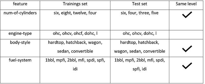
In the first step, we need to detect categorical features that have the same levels. The table above shows the num-of-cylinders feature in the training set and testing set has 4 and 4 levels. So, we keep it. The engine-type feature has no same level as the number of levels in the training and testing sets are 5 and 4 respectively. So, we remove this column. The body-style and fuel-system features, as you can see, both training and test set has 7 levels. So, they have same levels. After detecting the same level features, we need to ensure whether the classes are the same or not. In this case, the num-of-cylinders feature in the training set contains 4 different levels including six, eight, twelve, four. Comparing its classes with testing set’s shows that both datasets have six and four as classes. But in terms of two other classes, they are different. Therefore, we can jump to the conclusion the classes are not the same and we need to remove this feature. However, the situations for body-style and fuel-system features are different. Both have the same level and class simultaneously. Hence, the MCA platform can digest them now. Let’s see how we can make this process happen in the Python programming language.

def match(X_train_cat, X_test_cat):
    
    keep = X_train_cat.nunique() == X_test_cat.nunique()
    X_train_cat = X_train_cat[X_train_cat.columns[keep]]
    X_test_cat = X_test_cat[X_test_cat.columns[keep]]# For categorical features that have same levels, make sure the classes are the same
    keep = []
    for i in range(X_train_cat.shape[1]):
        keep.append(all(np.sort(X_train_cat.iloc[:,i].unique()) == np.sort(X_test_cat.iloc[:,i].unique())))
    X_train_cat = X_train_cat[X_train_cat.columns[keep]]
    X_test_cat = X_test_cat[X_test_cat.columns[keep]]
    
    return X_train_cat, X_test_cat

Build a Model

let’s suppose we want to predict the price of a car using categorical and numerical features. The purpose of the project is to build a supervised model using the 1985 Auto Imports dataset on the UCI repository. By running 10-fold cross-validation and tuning PCA and MCA techniques, we desire to build a regressor. To achieve that, after preprocessing the dataset, defining predictor and response variables, and splitting the dataset into training , validation and testing sets, we need to define the range of number of components for PCA and MCA as hyperparameters. To find the best regressor, we will find the best tuning parameters by applying training/validations analysis using mean squared error as an evaluation metric. The procedure is as follows. To better understanding the process, the pseudocode is as follows.

1- Split dataset into train/test sets

2- Define the tuning hyperparameters

3- For each fold of the the 10-fold cross-validation on the training set using KFold, complete remaining steps 4 through 11 for each iteration of the hyperparameter pairs

4- Separate input dataset into categorical and numerical features

5- Level the categorical features

6- Scale the numerical data by applying standardization

7- Fit PCA on scaled numerical features in the training set, and reduce numerical features in both the train and test sets using the PCA parameters

8- Fit MCA on categorical features in the training set using MCA, and reduce categorical features in both the train and test sets using the MCA parameters

9- Combine the numerical and categorical features of the train and test sets using the Concat function from the Pandas library

10- Fit a regression model on the train set

11- Report average MSE on the test set for each hyperparameter pair

12- Select the hyperparameter pair that has the best (lowest) MSE and fit the final dimension reduction/regression model on the full training data

13- Report the MSE on testing set using the reduced dimensions

Conclusion:

Based on the dataset, dimension reduction usually speeds up the training, but it may not always lead to a better or simpler solution. Also, There is a likely that we lose some information through MCA and PCA. To compare their results, building differenet models using original dataset would be a reasonable move.

Thank you for reading this article. This was an article focused on PCA, MCA, and building a model via tuning these feature reduction methods. You can find all the codes mentioned here on my Github page.

I am Sina Shariati, a data-savvy business analyst from San Francisco. Feel free to leave any ideas, comments, or concerns here or on my LinkedIn page.

Tune reduction techniques, PCA and MCA, to build a model on a mixed data

PCA

MCA

How to apply MCA and PCA on the Categorical and Numerical features

Build a Model

Conclusion:

Source:

Sign up to discover human stories that deepen your understanding of the world.

Free

Membership

Written by Sina Shariati

No responses yet